Problem Description:
Analyzing Socioeconomic Disparities in the US
The regression analysis assignment using SPSS involves interpreting and communicating key insights from census data on White-Asian income differences across four US regions. The focus is on identifying major trends in per capita income and presenting compelling headlines backed by data.
Per-Capita Income Disparities Across US Regions
According to Figure 1, significant disparities exist in per capita income across US regions. Notably, the northeast and west regions demonstrate higher per capita incomes for both White and Asian populations. However, White individuals generally exhibit higher per capita income compared to their Asian counterparts, except in the Northeast where Asian descent shows a lower per capita income.
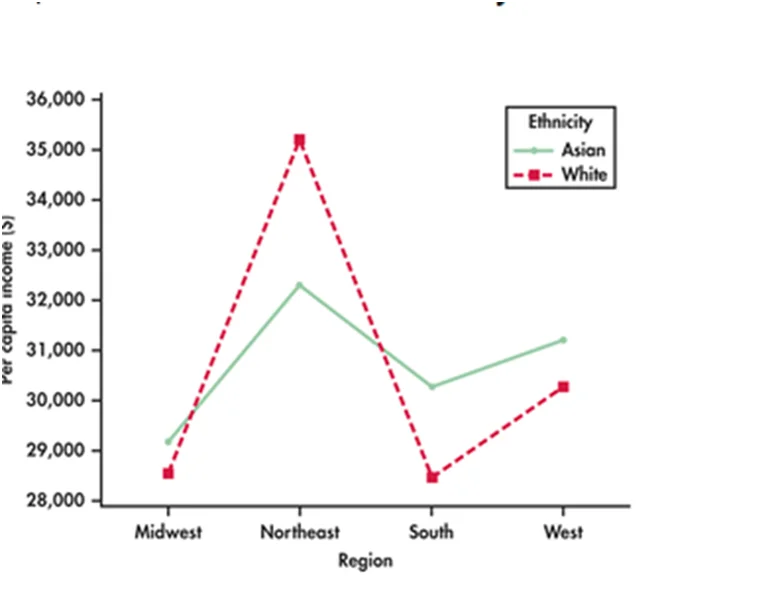
Figure 1: White-Asian Per Capita Income Disparities Across US Regions
Problem Description: Analyzing Educational Assessment Results
Figure 2 displays three-year longitudinal test results from National Assessments in Science, examining the performance of different age groups in physical and biological science. The assignment requires identifying the independent and dependent variables in a three-way ANOVA model and evaluating the main effects and interactions.
Solution: Understanding Three-Way ANOVA in Educational Assessments
In the three-way ANOVA model:
- Independent Variables:
- Age Level (9, 13, 17)
- Content Areas (Physical Science, Biological Science)
- Year (Year 1, Year 2, Year 3)
- Dependent Variable:
- The mean score on the science assessment test (percent of questions correct)
Significant main effects are observed across years on the mean score of the assessment test.
While there is no significant two-way interaction between age level and content area for ages 9 and 13, there is a significant interaction for age 17. Furthermore, a significant three-way interaction is identified for age 17, content, and year.
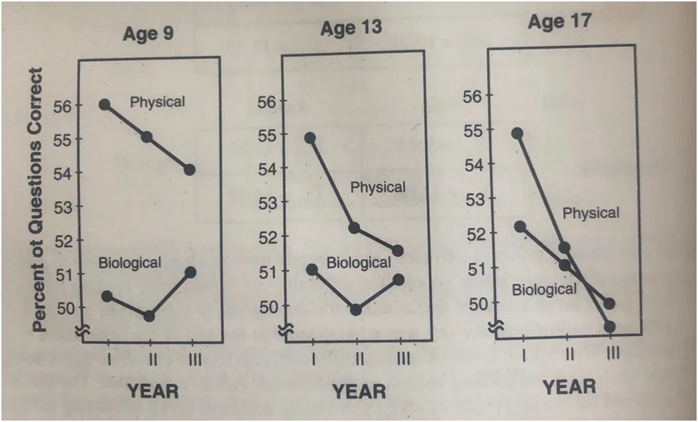
Figure 2: Three-Year Longitudinal Test Results from National Assessments in Science
Problem Description: Exploring Health Behavior Predictors Using Theory of Planned Behavior
The study applies the Theory of Planned Behavior (TPB) to understand people's intention to use non-pharmacological practices for chronic pain. Hierarchical linear regression is used to assess the contribution of TPB variables to predicting behavioral intention, above and beyond known patient background variables.
Solution: Predicting Behavioral Intention in Chronic Pain Treatment
In the hierarchical linear regression analysis:
- Model 1 (Background Variables):
- Explains 10.6% of the variation in behavioral intention.
- General anxiety disorder and education are significant predictors.
- Model 2 (TPB Construct):
- Explains 71.2% of the variation, showing a significant increase.
- Attitude direct, subjective norms and perceived behavioural control contribute significantly.
ANOVA tables confirm the overall model fits the data significantly in both models. Notably, general anxiety disorder is a consistent predictor of behavioural intention in both models.
Residual analysis confirms the fulfilment of normality and homogeneity variance assumptions.
Interpreting Linear Regression Analysis on Female Life Expectancy
Overview of the Analysis: The linear regression analysis aimed to predict female life expectancy (lifeexpf) across various countries using specific predictors: Percent urban population (urban), Infant mortality rate (infmr), Birth rate per 1,000 (birthrat), and Fertility rate per woman (fertrate). The analysis assessed the reliability of the model and, if needed, resolved any issues before interpretation.
Model Assessment: The model demonstrated no issues with normality or homogeneity of variance assumptions. The adjusted R^2 value of 0.949 indicates that 94.9% of the variation in female life expectancy in 1992 was explained by the independent variables.
Model Summary:
- Adjusted R^2: 0.949
- Significant Predictors: Fertility rate, Percent urban, Infant mortality rate, Births per 1000 population
- Overall Significance: F (4,114) = 548.029, p = 0.000
ANOVA Table:
| Model | Sum of Squares | df | Mean Square | F | Sig. | |
|---|---|---|---|---|---|---|
| 1 | Regression | 14362.034 | 4 | 3590.508 | 548.029 | .000b |
| Residual | 746.891 | 114 | 6.552 | |||
| Total | 15108.924 | 118 | ||||
| a. Dependent Variable: Female life expectancy 1992 | ||||||
| b. Predictors: (Constant), Fertility rate per woman, 1990, Percent urban, 1992, Infant mortality rate 1992 (per 1000 live births), Births per 1000 population, 1992 | ||||||
Table 1: ANOVA table used to check the overall model
- Significance: F (4,114) = 548.029, p = 0.000
Interpretation of Significant Predictors:
1. Percent Urban Population (1992):
- Statistically significant predictor.
- β = 0.047, t = 3.474, p < 0.05.
- For a one percent increase in urban population, female life expectancy increased by 0.047, holding other variables constant.
2. Births per 1000 Population (1992):
- Statistically significant predictor.
- β = -0.141, t = -2.120, p < 0.05.
- Each additional birth per 1000 population led to a decrease of 0.141 in female life expectancy, holding other variables constant.
3. Infant Mortality Rate (1992):
- Statistically significant predictor.
- β = -0.212, t = -18.964, p < 0.05.
- Each additional unit of infant mortality rate per 1000 live births resulted in a decrease of 0.212 in female life expectancy, holding other variables constant.
4. Fertility Rate per Woman (1990):
- Not statistically significant (p = 0.371).
Conclusion:
The linear regression model effectively explains female life expectancy in 1992 based on the selected predictors. Percent urban population, births per 1000 population, and infant mortality rate are significant contributors. The model provides valuable insights into the relationships between these factors and female life expectancy, aiding in informed decision-making for public health and policy interventions.
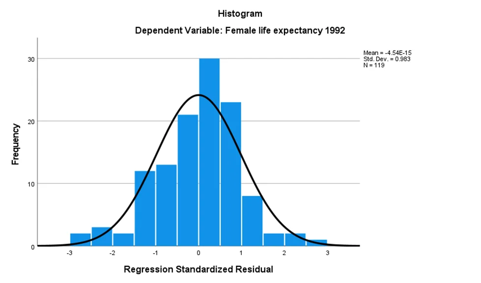
Chart 1: Female life expectancy graph
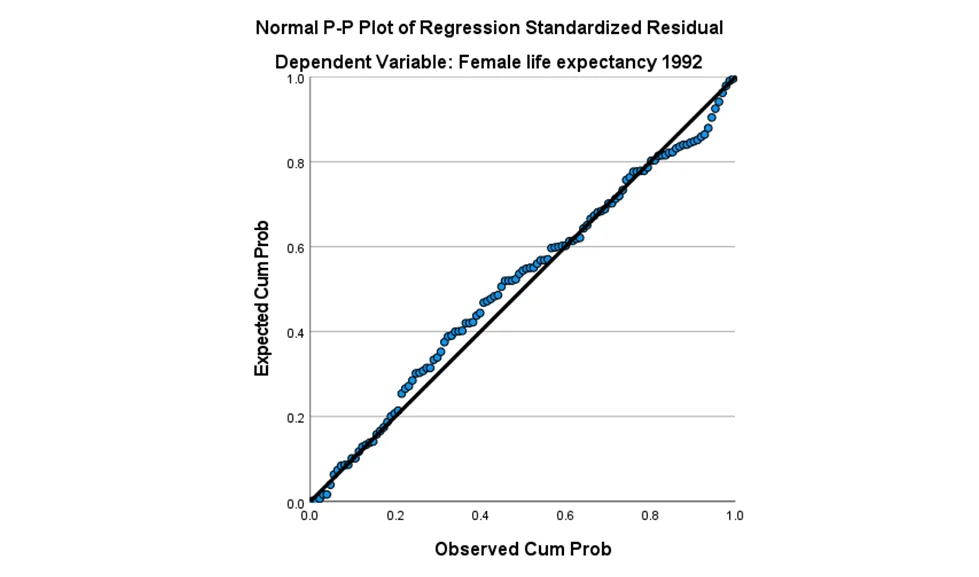
Chart 2: The observed vs. expected Cum probe of regression standardized residual
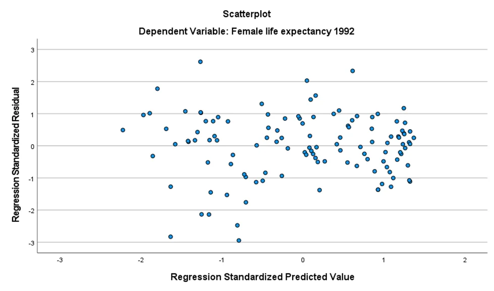
Chart 3: The predicted value for female life expectancy in 1992