Problem Description:
We investigate several hypotheses and conduct statistical tests to determine the relationships between different variables. We address questions related to education and smoking habits, responsibility for aging parents and political party identification, average test scores of affirmative action students and regular students, mean internet usage for male and female respondents, average days of poor mental health across different weight categories, and average enrollments in educational institutions across different regions in the country.
Solution:
One LURKING VARIABLE that may cause reversal in the direction of relationship between marital status and single is LEVEL OF EDUCATION. The reason for picking education level is that it is a proxy for skill. The higher the education level, the higher the skill and the higher the probability to get high-income job. It is possible that large proportion of married people have high educational qualification than single. This make sense as it is possible that most of college and university student working along with study are most likely single and they work in low-income job. If education level is not controlled for in the model, it will appear that income level is being affected by marital status.
Following the steps of hypothesis testing:
Step 1: State the Null and alternative hypothesis
- Ho: There is no significant association between level of education achieved and smoking
- H1: There is significant association between level of education achieved and smoking
Step 2: state the significance level
The level of significance (alpha) for this test is 0.05
Step 3: State the test statistics to be used
The relevant test statistics for the test is chi-square test because both dependent and independent variables are categorical variables.
Step 4: calculate the test statistics
The formula for chi-square is given as:
Where O is the observed frequency and E is the expected frequency.
The expected frequency is calculated as:
Where RT is the row total; CT is the column total and GT is the grand total.
The calculation is summarized in the table below:
| Education | Smoking | O | E | O-E | (O-E)^2 | (O-E)^2/E |
|---|---|---|---|---|---|---|
| High School | Nonsmoker | 56 | 59.48 | -3.48 | 12.12 | 0.20 |
| Former | 54 | 50.93 | 3.07 | 9.45 | 0.19 | |
| Moderate | 41 | 42.37 | -1.37 | 1.88 | 0.04 | |
| Heavy | 36 | 34.22 | 1.78 | 3.16 | 0.09 | |
| College | Nonsmoker | 37 | 44.21 | -7.21 | 52.03 | 1.18 |
| Former | 43 | 37.85 | 5.15 | 26.48 | 0.70 | |
| Moderate | 27 | 31.49 | -4.49 | 20.20 | 0.64 | |
| Heavy | 32 | 25.44 | 6.56 | 43.06 | 1.69 | |
| Graduate | Nonsmoker | 53 | 42.31 | 10.69 | 114.38 | 2.70 |
| Former | 28 | 36.22 | -8.22 | 67.57 | 1.87 | |
| Moderate | 36 | 30.14 | 5.86 | 34.40 | 1.14 | |
| Heavy | 16 | 24.34 | -8.34 | 69.55 | 2.86 | |
| 2=13.30 |
From the calculation, the test statistics χ^2=13.30
Step 5: calculate the Critical Value and calculate the p-value
The critical value of χ^2 (α,df)=χ^2 (0.05,6)=12.59
df=(r-1)(c-1)
Where r is the number of levels in education and c is the number of levels in smoking. Thus r is 3 and c is 4. Thus df=(3-1)(4-1)=6
The p-value is 0.039
Step 6: state the decision criteria
If the test statistics is greater than the critical value or the p-value is less than the level of significance (α=0.05), we reject the null hypothesis while if the test statistics is less than the critical value or the p-value is greater than the level of significance (α=0.05) we do not reject the null hypothesis.
Step 7: State the decision
The test statistics (13.3) is greater than the critical value (12.59) and the p-value (0.039) is less than the level of significance (α=0.05). Therefore, we reject the null hypothesis that there is no significant association between level of education achieved and smoking. We conclude there is significant association between level of education achieved and smoking.
Step 8: State the conclusion
Since there is significant association between level of education achieved and smoking, we conclude that the pattern of relationship between smoking and level of education has not changed.
3 DATA WORK
Following the steps of hypothesis testing:
Step 1: State the Null and alternative hypothesis
- Ho: There is no significant association between opinion on responsibility for aging parent (KIDPARS) and political party identification
- H1: There is no significant association between opinion on responsibility for aging parent (KIDPARS) and political party identification
Step 2: state the significance level
The level of significance (alpha) for this test is 0.01
Step 3: State the test statistics to be used
The relevant test statistics for the test is chi-square test because both dependent and independent variables are categorical variables.
Step 4: calculate the test statistics
The formula for chi-square is given as:
Where O is the observed frequency and E is the expected frequency.
The expected frequency is calculated as:
Where RT is the row total; CT is the column total and GT is the grand total.
The result from SPSS is presented below
Chi-Square Tests
| Value | df | Asymp. Sig. (2-sided) | |
|---|---|---|---|
| Pearson Chi-Square | 54.777a | 28 | .002 |
| Likelihood Ratio | 63.153 | 28 | .000 |
| Linear-by-Linear Association | 5.353 | 1 | .021 |
| N of Valid Cases | 2261 |
4 cells (10.0%) have expected count less than 5. The minimum expected count is 1.10.
From the result, the test statistics χ^2=54.78
Step 5: calculate the Critical Value and calculate the p-value
The critical value of χ^2 (α,df)=χ^2 (0.01,28)=48.28
df=(r-1)(c-1)
Where r is the number of levels in education and c is the number of levels in smoking. Thus r is 3 and c is 4. Thus df=(5-1)(8-1)=28
The p-value from the result is 0.002
Step 6: state the decision criteria
If the test statistics is greater than the critical value or the p-value is less than the level of significance (α=0.01), we reject the null hypothesis while if the test statistics is less than the critical value or the p-value is greater than the level of significance (α=0.01) we do not reject the null hypothesis.
Step 7: State the decision
The test statistics (54.78) is greater than the critical value (48.28) and the p-value (0.002) is less than the level of significance (α=0.01). Therefore, we reject the null hypothesis that there is no significant association between opinion on responsibility for aging parent (KIDPARS) and political party identification. We conclude there is significant association between opinion on responsibility for aging parent (KIDPARS) and political party identification
Step 8: State the conclusion
Since there is significant association between pinion on responsibility for aging parent (KIDPARS) and political party identification, we conclude that there is sufficient evidence that opinion on responsibility for aging parents are diversed depending on political party affiliation.
Following the steps of hypothesis testing:
Step 1: State the Null and alternative hypothesis
- Ho: μ_RS=μ_AAS (there is no significant difference in mean score of affirmative action student and regular student)
- Ho: μ_RS≠μ_AAS (there is significant difference in mean score of affirmative action student and regular student)
Step 2: state the significance level
The level of significance (alpha) for this test is 0.05
Step 3: State the test statistics to be used
The relevant test statistics for the test is two sample Z-test because population standard deviation is known and the samples come from population that is normally distributed
Step 4: calculate the test statistics
The formula for two sample z-test statistics is:
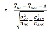
Where X ̅_RS Is the average score for regular students and X ̅_AAS is the average score of affirmative action student, Δ is the hypothesized mean difference which is zero in our case; σ_RS^2 is the population variance of regular student and σ_AAS^2 is the population variance of affirmative action students. n_RS and n_AAS are the sample size for regular and affirmative action students respectively.
From the data given: X ̅_RS=86.4,X ̅_AAS=84.1, σ_RS^2=〖17.3〗^2 σ_AAS^2=〖28.2〗^2, n_RS=44 n_AAS=19
Thus,
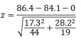
z=0.33
Step 5: calculate the Critical Value and calculate the p-value
The critical value of z_(α/2)=z_(0.05/2)=1.96
The p-value from the result is 0.63
Step 6: state the decision criteria
If the test statistics is greater than the critical value or the p-value is less than the level of significance (α=0.05), we reject the null hypothesis while if the test statistics is less than the critical value or the p-value is greater than the level of significance (α=0.05) we do not reject the null hypothesis.
Step 7: State the decision
The test statistics (0.33) is less than the critical value (1.96) and the p-value (0.63) is greater than the level of significance (α=0.05). Therefore, we do not reject the null hypothesis that there is no significant difference in average score of regular students and affirmative student. Thus, there is no significant difference in average score of regular students and affirmative student
Step 8: State the conclusion
Since there is no significant significant difference in average score of regular students and affirmative student. we conclude that there is no sufficient evidence to reject the claim that affirmative action students obtained a similar score in the state civil exam compared to regular students
Following the steps of hypothesis testing:
Step 1: State the Null and alternative hypothesis
- Ho: μ_male=μ_female (there is no significant difference in mean internet hours of male and female)
- Ho: μ_male>μ_female (mean internet hours of male is significantly greater than that of female)
Step 2: state the significance level
The level of significance (alpha) for this test is 0.05
Step 3: State the test statistics to be used
The relevant test statistics for the test is two sample t-test because sample standard deviation is known.
Step 4: calculate the test statistics
The formula for two sample z-test statistics is:
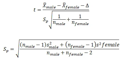
Where X ̅_male Is the average internet time for male and X ̅_female is the average internet time for female, Δ is the hypothesized mean difference which is zero in our case; s_male^2 is the sample standard deviation of male and s_female^2 is the sample standard deviation of female. n_male and n_female are the sample size for male and female respectively.
From the data given: X ̅_male=10.17,X ̅_female=9.08, s_male^2=〖12.26〗^2 s_female^2=〖11.71〗^2, n_male=118 n_female=157
Thus,
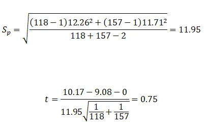
t=0.75
Step 5: calculate the Critical Value and calculate the p-value
The critical value of t(α,df)=t(0.05,273)=1.65
df=n_1+n_2-2=118+157-2=273
The p-value from the result is 0.45
Step 6: state the decision criteria
If the test statistics is greater than the critical value or the p-value is less than the level of significance (α=0.05), we reject the null hypothesis while if the test statistics is less than the critical value or the p-value is greater than the level of significance (α=0.05) we do not reject the null hypothesis.
Step 7: State the decision
The test statistics (0.75) is less than the critical value (1.65) and the p-value (0.45) is greater than the level of significance (α=0.05). Therefore, we do not reject the null hypothesis that there is no significant difference in average internet use of male and female. Thus, there is no significant difference in average internet use of male and female.
Step 8: State the conclusion
Since there is no significant difference in average internet use of male and female. We conclude that there is no sufficient evidence to support the claim that men use the internet more hours than women.
Using alpha value of 0.01; the critical value becomes t(α,df)=t(0.01,273)=2.34 but the test statistics and p-values remain 0.75 and 0.45 respectively. Since The test statistics (0.75) is less than the critical value (1.65) and the p-value (0.45) is greater than the level of significance (α=0.01). Therefore, we do not reject the null hypothesis that there is no significant difference in average internet use of male and female at 1% level of significance. Thus, there is no significant difference in average internet use of male and female at 1% level of significance.
Conlusion at α=0.01
Since there is no significant difference in average internet use of male and female at α=0.01. We conclude that there is no sufficient evidence to support the claim that men use the internet more hours than women.
Therefore, the decision is not different if alpha was set at 0.01
Following the steps of hypothesis testing:
Step 1: State the Null and alternative hypothesis
- Ho: μ_RW=μ_VO (there is no significant difference in mean days of poor mental health in the last 30 days of rightly weight and Very overweight respondents)
- Ho: μ_RW≠μ_VO (there is significant difference in mean days of poor mental health in the last 30 days of rightly weight and very overweight respondents)
Step 2: state the significance level
The level of significance (alpha) for this test is 0.05
Step 3: State the test statistics to be used
The relevant test statistics for the test is two sample t-test because sample standard deviation is known
Step 4: calculate the test statistics
The result from SPSS is shown below
Group Statistics
| R weight rating | N | Mean | Std. Deviation | Std. Error Mean | |
|---|---|---|---|---|---|
| Days of poor physical health past 30 days | ABOUT THE RIGHT WEIGHT | 730 | 2.36 | 5.615 | .208 |
| VERY OVERWEIGHT | 91 | 4.97 | 9.168 | .961 |
Independent Samples Test
| Levene's Test for Equality of Variances | t-test for Equality of Means | |||||||||
|---|---|---|---|---|---|---|---|---|---|---|
| F | Sig. | t | df | Sig. (2-tailed) | Mean Difference | Std. Error Difference | 95% Confidence Interval of the Difference | |||
| Lower | Upper | |||||||||
| Days of poor physical health past 30 days | Equal variances assumed | 28.588 | .000 | -3.833 | 819 | .000 | -2.603 | .679 | -3.935 | -1.270 |
| Equal variances not assumed | -2.647 | 98.585 | .009 | -2.603 | .983 | -4.554 | -.651 | |||
The tests statistics is -2.647. This test statistics is chose because we could not assume equal variance as the F stat result showed rejection of the null hypothesis of equal variance.
Step 5: calculate the Critical Value and calculate the p-value
The critical value of t(α,df)=t(0.05,95.585)=-1.66
The p-value from the result is 0.009
Step 6: state the decision criteria
If the test statistics is greater than the critical value or the p-value is less than the level of significance (α=0.05), we reject the null hypothesis while if the test statistics is less than the critical value or the p-value is greater than the level of significance (α=0.05) we do not reject the null hypothesis.
Step 7: State the decision
The test statistics (-2.65) is greater than the critical value (-1.66) and the p-value (0.009) is less than the level of significance (α=0.05). Therefore, we do not reject the null hypothesis that the mean days of poor mental health in the last 30 days of rightly weight and very overweight. Thus, there is significant difference in mean days of poor mental health in the last 30 days of rightly weight and very overweight.
Step 8: State the conclusion
Since there is significant difference in average days of poor mental health in the last 30 days of rightly weight and overweight. We conclude that there is sufficient evidence to support the claim that there is significant difference in mean days of poor mental health in the last 30 days of rightly weight and very overweigt.
Following the steps of hypothesis testing:
Step 1: State the Null and alternative hypothesis
- Ho: μ_RW=μ_SO (there is no significant difference in mean days of poor mental health in the last 30 days of rightly weight and slightly overweight respondents)
- Ho: μ_RW≠μ_SO (there is significant difference in mean days of poor mental health in the last 30 days of rightly weight and slightly overweight respondents)
Step 2: state the significance level
The level of significance (alpha) for this test is 0.05
Step 3: State the test statistics to be used
The relevant test statistics for the test is two sample t-test because sample standard deviation is known
Step 4: calculate the test statistics
The result from SPSS is shown below
Group Statistics
| R weight rating | N | Mean | Std. Deviation | Std. Error Mean | |
|---|---|---|---|---|---|
| Days of poor physical health past 30 days | ABOUT THE RIGHT WEIGHT | 730 | 2.36 | 5.615 | .208 |
| SLIGHTLY OVERWEIGHT | 307 | 2.80 | 6.317 | .361 |
Independent Samples Test
| Levene's Test for Equality of Variances | t-test for Equality of Means | |||||||||
|---|---|---|---|---|---|---|---|---|---|---|
| F | Sig. | t | df | Sig. (2-tailed) | Mean Difference | Std. Error Difference | 95% Confidence Interval of the Difference | |||
| Lower | Upper | |||||||||
| Days of poor physical health past 30 days | Equal variances assumed | 1.952 | .163 | -1.110 | 1035 | .267 | -.440 | .397 | -1.219 | .338 |
| Equal variances not assumed | -1.058 | 519.025 | .291 | -.440 | .416 | -1.258 | .377 | |||
The tests statistics is -1.11. This test statistics is chose because we could assume equal variance as the F stat result showed non-rejection of the null hypothesis of equal variance.
Step 5: calculate the Critical Value and calculate the p-value
The critical value of t(α,df)=t(0.05,1035)=-1.65
The p-value from the result is 0.267
Step 6: state the decision criteria
If the test statistics is greater than the critical value or the p-value is less than the level of significance (α=0.05), we reject the null hypothesis while if the test statistics is less than the critical value or the p-value is greater than the level of significance (α=0.05) we do not reject the null hypothesis.
Step 7: State the decision
The test statistics (-1.11) is less than the critical value (-1.65) and the p-value (0.267) is greater than the level of significance (α=0.05). Therefore, we reject the null hypothesis that the mean days of poor mental health in the last 30 days of rightly weight and slightly overweight. Thus, there is no significant difference in mean days of poor mental health in the last 30 days of rightly weight and slightly overweight.
Step 8: State the conclusion
Since there is no significant difference in average days of poor mental health in the last 30 days of rightly weight and slightly overweight. We conclude that there is no sufficient evidence to support the claim that there is significant difference in mean days of poor mental health in the last 30 days of rightly weight and slightly overweight respondents.
Following the steps of hypothesis testing:
Step 1: State the Null and alternative hypothesis
- Ho: μ_West=μ_midwest=μ_Northeast=μ_South (there is no significant difference in average enrolments across different parts of the country)
- Ho: μ_West≠μ_midwest≠μ_Northeast≠μ_South (there is significant difference in average enrolments across different parts of the country)
Step 2: state the significance level
The level of significance (alpha) for this test is 0.05
Step 3: State the test statistics to be used
The relevant test statistics for the test is one-way ANOVA as there are more than two independent groups.
Step 4: calculate the test statistics
The result from SPSS is shown below
ANOVA
| enrolment | |||||
|---|---|---|---|---|---|
| Sum of Squares | df | Mean Square | F | Sig. | |
| Between Groups | 20.503 | 3 | 6.834 | 1.660 | .199 |
| Within Groups | 111.175 | 27 | 4.118 | ||
| Total | 131.677 | 30 | |||
The tests statistics is 1.66.
Step 5: calculate the Critical Value and calculate the p-value
The critical value of F(3,27)=2.96
The p-value from the result is 0.199
Step 6: state the decision criteria
If the test statistics is greater than the critical value or the p-value is less than the level of significance (α=0.05), we reject the null hypothesis while if the test statistics is less than the critical value or the p-value is greater than the level of significance (α=0.05) we do not reject the null hypothesis.
Step 7: State the decision
The test statistics (1.66) is less than the critical value (2.96) and the p-value (0.199) is greater than the level of significance (α=0.05). Therefore, we do not reject the null hypothesis that the average enrolment is the same across different part of the country. Thus, there is no significant difference in average enrolment across different part of the country.
Step 8: State the conclusion
Since there is no significant difference in average enrolment across different part of the country. We conclude that there is no sufficient evidence to support the claim that mean enrolments is different in all parts of the country.
Step 1: State the Null and alternative hypothesis
- Ho: μ_VO=μ_SO=μ_RW=μ_SU=μ_VU (there is no significant difference in average days of poor mental health in the past 30 days across categories of respondent’s weight)
- Ho: μ_VO≠μ_SO≠μ_RW≠μ_SU≠μ_VU (there is significant difference in average days of poor mental health in the past 30 days across categories of respondent’s weight)
Step 2: state the significance level
The level of significance (alpha) for this test is 0.05
Step 3: State the test statistics to be used
The relevant test statistics for the test is one-way ANOVA as there are more than two independent groups.
Step 4: calculate the test statistics
The result from SPSS is shown below
ANOVA
Days of poor mental health past 30 days
| Sum of Squares | df | Mean Square | F | Sig. | |
|---|---|---|---|---|---|
| Between Groups | 1446.809 | 4 | 361.702 | 7.085 | .000 |
| Within Groups | 113186.363 | 2217 | 51.054 | ||
| Total | 114633.172 | 2221 |
Multiple Comparisons
Dependent Variable: Days of poor mental health past 30 days
Tukey HSD
| (I) R weight rating | (J) R weight rating | Mean Difference (I-J) | Std. Error | Sig. | 95% Confidence Interval | |
|---|---|---|---|---|---|---|
| Lower Bound | Upper Bound | |||||
| VERY OVERWEIGHT | SLIGHTLY OVERWEIGHT | 1.370 | .653 | .221 | -.41 | 3.15 |
| ABOUT THE RIGHT WEIGHT | 2.551* | .616 | .000 | .87 | 4.23 | |
| SLIGHTLY UNDERWEIGHT | .950 | .822 | .777 | -1.29 | 3.20 | |
| VERY UNDERWEIGHT | .191 | 1.829 | 1.000 | -4.80 | 5.18 | |
| SLIGHTLY OVERWEIGHT | VERY OVERWEIGHT | -1.370 | .653 | .221 | -3.15 | .41 |
| ABOUT THE RIGHT WEIGHT | 1.181* | .353 | .008 | .22 | 2.15 | |
| SLIGHTLY UNDERWEIGHT | -.420 | .649 | .967 | -2.19 | 1.35 | |
| VERY UNDERWEIGHT | -1.180 | 1.758 | .963 | -5.98 | 3.62 | |
| ABOUT THE RIGHT WEIGHT | VERY OVERWEIGHT | -2.551* | .616 | .000 | -4.23 | -.87 |
| SLIGHTLY OVERWEIGHT | -1.181* | .353 | .008 | -2.15 | -.22 | |
| SLIGHTLY UNDERWEIGHT | -1.601 | .612 | .068 | -3.27 | .07 | |
| VERY UNDERWEIGHT | -2.360 | 1.744 | .658 | -7.12 | 2.40 | |
| SLIGHTLY UNDERWEIGHT | VERY OVERWEIGHT | -.950 | .822 | .777 | -3.20 | 1.29 |
| SLIGHTLY OVERWEIGHT | .420 | .649 | .967 | -1.35 | 2.19 | |
| ABOUT THE RIGHT WEIGHT | 1.601 | .612 | .068 | -.07 | 3.27 | |
| VERY UNDERWEIGHT | -.760 | 1.827 | .994 | -5.75 | 4.23 | |
| VERY UNDERWEIGHT | VERY OVERWEIGHT | -.191 | 1.829 | 1.000 | -5.18 | 4.80 |
| SLIGHTLY OVERWEIGHT | 1.180 | 1.758 | .963 | -3.62 | 5.98 | |
| ABOUT THE RIGHT WEIGHT | 2.360 | 1.744 | .658 | -2.40 | 7.12 | |
| SLIGHTLY UNDERWEIGHT | .760 | 1.827 | .994 | -4.23 | 5.75 | |
The mean difference is significant at the 0.05 level.
The tests statistics is 7.085
Step 5: calculate the Critical Value and calculate the p-value
The critical value of F(4,2217)=2.38
The p-value from the result is <.001
Step 6: state the decision criteria
If the test statistics is greater than the critical value or the p-value is less than the level of significance (α=0.05), we reject the null hypothesis while if the test statistics is less than the critical value or the p-value is greater than the level of significance (α=0.05) we do not reject the null hypothesis.
Step 7: State the decision
The test statistics (7.085) is greater than the critical value (2.38) and the p-value (<.001) is greater than the level of significance (α=0.05). Therefore, we reject the null hypothesis that there is no significant difference in average days of poor mental health in the past 30 days across categories of respondent’s weight. Thus, there is significant difference in average days of poor mental health in the past 30 days across categories of respondent’s weight.
Since there is significant difference, Tukey HSD was used to determine which group is difference and it was found that there is significant difference between average days of poor mental health in the past 30 days of respondents with about the right weight and average days of poor mental health in the past 30 days of respondents with very overweight (p<.001). Also, there is significant difference between average days of poor mental health in the past 30 days of respondents with about the right weight and average days of poor mental health in the past 30 days of respondents with slightly overweight (p=0.008). There is no significant difference between other pairs
Step 8: State the conclusion
Since there is significant difference in average days of poor mental health in the past 30 days across categories of respondent’s weight. We conclude that there is sufficient evidence to support the claim that there is significant difference in average days of poor mental health in the past 30 days across categories of respondent’s weight.