Problem Description:
This R assignment delves into the exploration of determinants of income inequality in American states using a cross-sectional dataset named inequality.csv. The dataset provides information on income inequality in 50 American states in the year 2016. The dependent variable of interest is the Gini coefficient (gini), representing income inequality on a scale from 0 (perfect equality) to 1 (perfect inequality). The task is to select three independent variables from the provided list and perform correlation analysis, regression analysis, and regression diagnostics to understand their impact on income inequality.
Data
1. Selecting Variables: Analyze income inequality using the following independent variables:
- unemp: Unemployment rate (% of labor force).
- demgov: Dummy variable for Democratic governorship (1 for Democratic, 0 otherwise).
- minimumwage: State's statutory minimum wage (hourly rate in dollars).
2. Justification: Briefly explain why these variables are chosen and how they might influence income inequality.
3. Correlation Analysis: Compute Pearson's correlation coefficient for each pair of variables.
4. Scatter Plots: Create scatter plots between each independent variable and the dependent variable.
Homework Requirements
Problem Description: Define the Ordinary Least Squares (OLS) method and list assumptions for it to produce Best Linear Unbiased Estimators (BLUE).
Answer:
OLS Method: The Ordinary Least Squares (OLS) method is a statistical technique used for estimating parameters in a linear regression model.
Assumptions:
- Independence of individual outcomes.
- Equal variance of outcomes.
- The linear relationship between the outcome and independent variables.
2. Motivations for Multiple Regressions:
Problem Description: Explore the two major motivations behind running multiple regressions in comparison with simple linear regressions.
Answer:
- Including Multiple Predictors: Multiple regression allows the inclusion of multiple predictors, useful when the dependent variable is influenced by more than one predictor.
- Controlling for Confounding Variables: Multiple regression helps control for the effects of variables, not of primary interest but related to the dependent variable.
3. Regression Diagnostics:
Problem Description: Based on the regression diagnostics lecture, answer questions about influential points (A, B, C), their discrepancies, leverage, and influence.
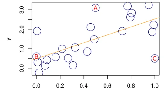
Figure 1: influential points and their discrepancies, leverage, and influence.
Answer:
- Discrepancy: Points A and C have discrepancies, being far from the regression line.
- Leverage: Point B has leverage as it lies on the line, affecting the determination of coefficients.
- Influence: Point C has influence, leading the regression line downward.
4. Selected Variables and Explanation:
Problem Description: Explain the rationale behind selecting the unemployment rate (unemp), the nature of the state's government (demgov), and the minimum wage variable for analyzing income inequality in American states. Justify the significance of each variable in influencing income distribution succinctly.
Answer: For the analysis of income inequality in American states, three crucial variables were chosen: the unemployment rate (unemp), the nature of the state's government (demgov), and the minimum wage variable. The unemployment rate is considered a significant factor influencing income inequality, as higher employment correlates with more resources favouring the employed, thereby contributing to unequal distribution. The political nature of the state, indicated by demgov, is another key influencer, as government policies play a pivotal role in shaping income distribution. Finally, the minimum wage variable is essential, as it determines the wage at which industrialists and firms can hire individuals, impacting the overall income inequality by influencing profit distribution.
4.1 Pearson’s Correlation Coefficient:
Problem Description: Compute Pearson’s correlation coefficient for the Gini index and selected independent variables (unemp, demgov, minimumwage). Present the correlation matrix and interpret the results, emphasizing the implications of the coefficients on the analysis of income inequality.
Answer: To quantify the relationships, the Pearson’s correlation coefficient was computed for each pair of variables, including the dependent variable (gini) and the selected independent variables (unemp, demgov, minimumwage). The correlation matrix indicates the strength and direction of these relationships. Notably, the correlation coefficients suggest a positive correlation between the Gini index and both the unemployment rate and the minimum wage, while the nature of the state's government exhibits a weaker positive correlation.
4.2 Scatter Plots and Relationship Assessment:
Problem Description: Create scatter plots for each independent variable against the Gini index. Interpret the visual representations, indicating positive or negative relationships. Discuss the significance of these observations in the broader context of analyzing income inequality in American states.
Answer: Scatter plots were generated to visually assess the relationship between each independent variable and the dependent variable (Gini index). The plot of the unemployment rate against the Gini index reveals a positive relationship, supporting the idea that higher unemployment rates contribute to increased income inequality. Similarly, the scatter plot for the nature of the state's government (demgov) and Gini index displays a positive trend. Lastly, the scatter plot for minimum wage and the Gini index suggests a positive relationship, indicating that higher minimum wages may contribute to greater income inequality.
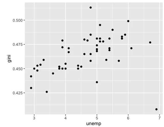
Graph 1: The relationship between Gini and Unemp.
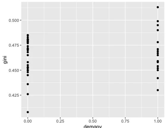
Graph 2: The relationship between Gini and Demgov
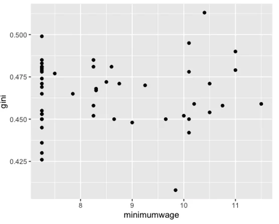
Graph 3: The relationship between Gini and Minimumwage
5. Regression Analysis
5.1 Estimate a Multiple Regression Model
Problem Description: Estimate a multiple regression model and present regression results in a table
Regression Results:
lin=lm(gini~.,data=df)
summary(lin)
##
## Call:
## lm(formula = gini ~ ., data = df)
##
## Residuals:
##       Min        1Q    Median        3Q       Max
## -0.073636 -0.007868  0.001663  0.011059  0.042650
##
## Coefficients:
##               Estimate Std. Error t value Pr(>|t|)
## (Intercept)  0.4254520  0.0208715  20.384  < 2e-16 ***
## unemp        0.0086718  0.0026331   3.293  0.00191 **
## demgov       0.0071324  0.0059420   1.200  0.23615
## minimumwage -0.0003711  0.0020551  -0.181  0.85749
## ---
## Signif. codes:  0 '***' 0.001 '**' 0.01 '*' 0.05 '.' 0.1 ' ' 1
##
## Residual standard error: 0.01805 on 46 degrees of freedom
## Multiple R-squared:  0.1996, Adjusted R-squared:  0.1474
## F-statistic: 3.825 on 3 and 46 DF,  p-value: 0.0158
Interpretation:
- Only the variable "unemp" is statistically significant.
- For a one percent increase in unemployment, the Gini index increases by 0.0086718.
5.2 Interpretation of Regression Coefficients
Problem Description: Are all three regression coefficients significant or not? Interpret the three slope coefficients substantively.
Answer: Not all three variables are significant. Only the "unemp" variable is statistically significant. For a one percent increase in unemployment, the Gini index increases by 0.0086718.
6. Regression Diagnostics
6.1 Residuals vs. Fitted Values Plot
Problem description: Create a two-way scatter plot to see if the mean of residuals is centered around zero across all fitted values.
Residuals <- resid(lin)
fitted_values <- fitted(lin)
plot(fitted_values, residuals, main = "Residuals vs Fitted Values", xlab = "Fitted Values", ylab = "Residuals")
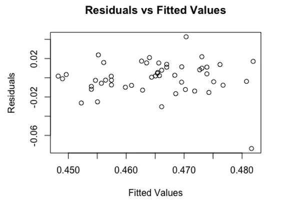
Figure 2: Residual against fitted values
Interpretation: The plot indicates that the mean of residuals is centered around zero across all fitted values.
6.2 Multicollinearity Check
Problem Description: Is there multicollinearity? Answer this question based on variance inflation factors (VIFs).
Answer:
library(car)
## Warning: package 'car' was built under R version 4.1.2
## Loading required package: carData
## Warning: package 'carData' was built under R version 4.1.2
vif(lin)
##       unemp      demgov minimumwage
##    1.019954    1.216245    1.194648
Interpretation: As the VIF does not cross 5 for any variable, we conclude that there is no multicollinearity.
7. Bonus Points
7.1 Identify Influential Points
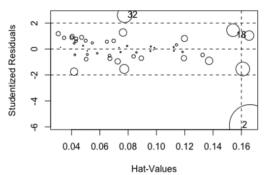
Problem Description: Are there any influential points that disproportionately drive the regression results? Please create an influence plot to identify influential points.
Answer:
Figure 3: Studentized residuals vs. hat values
Interpretation: Point number 32 is identified as an influential point.
7.2 Remove Influential Point and Reestimate Regression
df1=df[-32,]
lin1=lm(gini~.,data=df1)
summary(lin1)
##
## Call:
## lm(formula = gini ~ ., data = df1)
##
## Residuals:
##       Min        1Q    Median        3Q       Max
## -0.071771 -0.008398  0.001523  0.010551  0.025459
##
## Coefficients:
##              Estimate Std. Error t value Pr(>|t|)
## (Intercept)  0.432444   0.019846  21.790  < 2e-16 ***
## unemp        0.008341   0.002484   3.358  0.00161 **
## demgov       0.005090   0.005653   0.900  0.37265
## minimumwage -0.001039   0.001953  -0.532  0.59720
## ---
## Signif. codes:  0 '***' 0.001 '**' 0.01 '*' 0.05 '.' 0.1 ' ' 1
##
## Residual standard error: 0.017 on 45 degrees of freedom
## Multiple R-squared:  0.2048, Adjusted R-squared:  0.1518
## F-statistic: 3.863 on 3 and 45 DF,  p-value: 0.0153
Comparison: Comparing the new regression with the original one, the coefficients and significance levels change slightly, suggesting that the influential point had some impact on the results.