Problem Description:
The data analysis assignment at hand involves conducting exploratory data analysis (EDA) and data preparation in RapidMiner for a dataset related to predicting whether it will rain tomorrow. The dataset includes various features such as temperature, humidity, rainfall, and location, which are used to predict the binary target variable - whether it will rain the following day. The analysis involves examining data distributions, correlations, and preparing the dataset for model building.
Solution
Task 1.1 Exploratory data analysis and data preparation
Figure 1 displays two graphs: scatter plot of target variable vs date (left) and histogram of target variable
 and histogram of target variable.webp)
Figure 1
(right). From scatter plot we see that data acquired in 2017 is missing. Histograms informs us that that target variable distribution is unbalanced number of “No” is 5x times more than “Yes”, also there are some missing values denoted as “N/A”.
Figure 2 shows that amount of collected data in every year is nearly the same except 2008 and 2017.
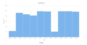
Figure 2: Date histogram
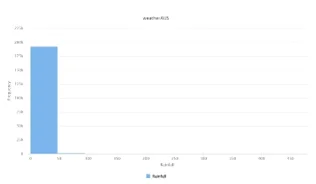
Figure 3: Histogram of Rainfall
From figure 3(histogram of rainfall) we see that the data is very unbalanced. Similar histograms have “Evaporation” and “Risk_mm”.
From figure 4 (Location vs Target Variable) we see that except “Nhil” and Uluru number of predictions about tomorrow raining are nearly the same in every state. A good idea is to check tomorrow rain prediction of different states and see if some states are rainier that others.
.webp)
Figure 4: Location vs target variable (Will tomorrow rain on not ?)
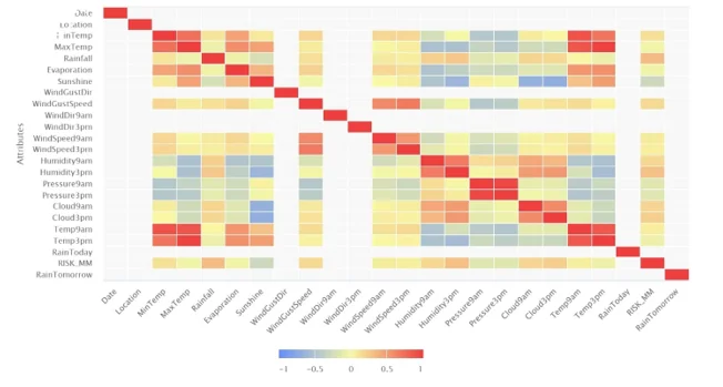
Figure 5: Correlation Matrix
From correlation matrix we see that highly correlated features are: (Temp 9am,Mintemp),(Temp3 pm, maxtemp), (Min temp,Maxtemp), (Temp 9 am, Temp 3 am),( Pressure 9 am, Pressure 3 am). Therefore, we can remove Mintemp, Maxtemp, Temp 9 am, Pressure 3 pm.
We can also remove Date and Location column because they are not informative to the model. Date would be informative in time series prediction. Location also is not informative because rain will be tomorrow or not mainly is defined by temperature, humidity, sunshine and other variables. Also, Location variable has too many categories which very complicates dataset dimensionality I have removed them.
Missing values in categorical columns were filled using statistical mode and numerical columns with statistical mean or average value.
After removing unnecessary columns which were highly correlated to each other the obtain correlation matrix is shown on figure 6
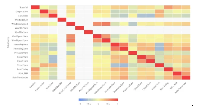
Figure 6: new correlation matrix obtained after removing highly correlated features
As we see from the correlation’s matrix the most important parameters to predict the target variable are: RISL_MM, humidity 3 pm, “RainToday”, “Rainall” and “windguest” speed.
Variables related to cloud are integers and have value from 1- to 10. Some may think that this variable is categorical but according to the descriptions they are the fraction of the sky obscured at some predefined time during day (specifically 3 pm and 9 am). Therefore, this variable is numerical in nature. Higher values are MORE in value that lower ones, which is not the case of categorical variables. The only transformation applied to the variables are data normalization using Z-transformation. Model converges well when it is trained on the training set. Also feature engineering was not needed because I did not see the connection or combination between variables which can be more correlated to the target variable than they itself. I have converted target variable into binomial variable because it is categorical variable rather than numeric.
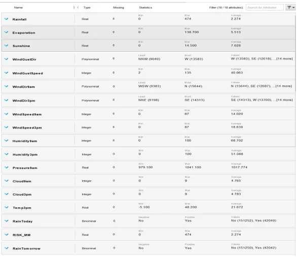
Table 1 shows the result of exploratory data analysis and data preparation done.
Task 1.1 Results of Exploratory Data Analysis and Data Preparation.
Task 1.2 Decision Tree Model
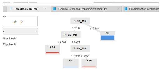
Trained decision Rapid Miner Tree
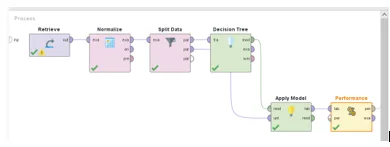
Decision Tree Rapid Miner process
Decision Tree Rapid Miner rules
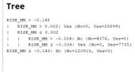
As we see from the diagrams important variable for decision tree is RISK_MM. All the other variables are not important for the tree to predict if rain will be tomorrow or not. This result makes sense because RISK_MM input feature (continuous feature) has a high correlation with target variable(will tomorrow rain or not?). Decision tree has gained most of the information from the RISK_MM. The performance of the Decision Tree model is given on the below figure.
The model has 100% accuracy on the test set. The decision tree model has 100% precision and 100% recall also it’s F1 score is 1.0. Elimination of different variables like ‘Data’, ‘Location’ and other highly correlated variables is justified by the result of the decision tree. If that variables were important than decision tree in no way would be able to achieve such a perfect result on training set.
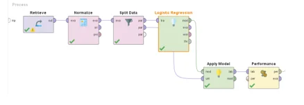
Task 1.3 Logistic Regression Model
Logistic Regression Rapid Miner process:
Logistic Regression Model Rapid Miner Key outputs
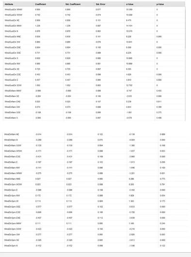
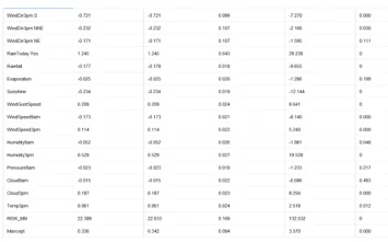
As we see from the above table the RISK_MM is the most important parameter for logistic regression model. The coefficient value for RISK_MM is 22.389 which is at least 20 times bigger than other coefficients. Some coefficients are negative, and some are positive. Positive coefficients mean than if input feature increases target variable increases, negative correlation means that target variable is decreased when input variable is increased.
Figure below displays the confusion matrix of trained Logistic Regression model on the test set.
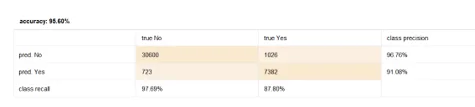
As we see logistic regression model precision is more on “No” class but “NO” class has higher recall.
Task 1.4 Model Validation and Performance
Decision Tree and Logistic Regression models were trained and tested using Cross-Validation method. The Cross validation on each iteration chooses different subset of dataset for training and validation. Normally Cross Validation performs 5 iterations. On each iteration dataset is divided into 5 subsets. One subset is sed for validation purposes and other 4 are used for training the model. After training the Final Decision Tree Model and the Final Logistic Regression model the models were compared: sing following model performance metrics (1) accuracy (2) sensitivity (3) specificity and (4) F1 score.
Table 1.4 The comparison of the final Decision Tree and the final Logistic Regression models in different performance metrics of classifier model.
Model |
Decision Tree |
Logistic Regression |
|---|---|---|
| Accuracy | 100.00% | 95.40% |
| Sensitivity | 100.00% | 87.87% |
| Specificity | 100.00% | 97.42% |
| F1 score | 100.00% | 88.98% |
As we see from the table 1.4 the Decision Tree model is better in every aspect over Logistic Regression Model. The Decision tree model is ideal it has no drawbacks. But logistic regression model is not bad, it is very good, performance measure metric value of every aspect is more than 88%. The Logistic Regression Model best parameter is specificity 97.42% which is very good result.