Problem Description:
This regression analysis assignment involves various regression analyses to model different scenarios. Here are the solutions presented in a more structured and organized manner:
1. Estimating the Rate of Return from Holding a Bottle of Wine:
Problem Description:
Which mathematical form of model (linear, semi-log, or double log) would be appropriate for estimating the rate of return from holding a bottle of wine for a year?
Answer: A semi-log model would be appropriate for estimating the rate of return from holding a bottle of wine for a year.
2. Predicting Children’s Weight:
Problem Description:
Imagine children’s weight has been estimated using the following equation for children aged 0 through 18.
Equation:WEIGHTi = 8.6 + 5.0AGEi + 0.4HEIGHTi + 9.0MALEi
A. Other things being the same, how does a child’s predicted weight increase as he ages by one year?
Answer: Other things being the same, the child’s predicted weight will increase by 5.0 as he ages by one year.
B. Why might multicollinearity be an issue with this model?
Answer: Multicollinearity might be an issue with this model because AGE and HEIGHT, as independent variables, are highly correlated.
3. Kaizen Processes and Employee Happiness:
Problem Description:
At Vermeer Farm and Construction in Iowa, they’re totally into Kaizen processes. Part of the reason that they like this is that a recent analysis of their employees showed that those who had participated in a Kaizen process at the company are happier employees.
A. Does this necessarily prove that Kaizen participation makes employees happier?
Answer: Yes, Kaizen participation makes employees happier because the process assures the complete participation of employees. It includes employees of all positions during kaizen activities.
B. Which underlying assumption of regression analysis is most likely violated in this situation?
Answer: Multicollinearity is most likely violated in this situation.
4. Linear Regression of Daily Stock Market Return:
Problem Description:
Here are some results from a linear regression of daily stock market return on daily trading volume.
Linear Regression of Return on Volume
| Model Summaryb | ||||||||||||
|---|---|---|---|---|---|---|---|---|---|---|---|---|
| Model | R | R Square | Adjusted R Square | Std. Error of the Estimate | Durbin-Watson | |||||||
| 1 | .029a | .001 | .000 | .0098957 | 2.155 | |||||||
| Table 1: linear regression on model summary a. Predictors: (Constant), Volume |
||||||||||||
| b. Dependent Variable: Return | ||||||||||||
| ANOVAa | ||||||||||||
| Model | Sum of Squares | df | Mean Square | F | Sig. | |||||||
| 1 | Regression | .000 | 1 | .000 | .718 | .397b | ||||||
| Residual | .081 | 829 | .000 | |||||||||
| Total | .081 | 830 | ||||||||||
| Table 2: Linear regression on ANOVA a. Dependent Variable: Return |
||||||||||||
| b. Predictors: (Constant), Volume | ||||||||||||
Coefficients
| Unstandardized Coefficients | Standardized Coefficients | t | Sig. | |
|---|---|---|---|---|
| B | Std. Error | Beta | ||
| .002 | .002 | 1.148 | .251 | |
| -3.820E-13 | .000 | -.029 | -.847 | .397 |
Table 3: The coefficients
A. How much explanatory power does this model have?
Answer: The model has 0.001 explanatory power, which is almost no power.
B. What does the estimated Durbin-Watson statistic suggest about serial correlation in the model?
Answer: Since the estimated Durbin-Watson statistic is greater than two, this suggests a negative serial correlation in the model.
C. The reported p-value for the F-test is 0.397. What is the interpretation of this result?
Answer: Since the p-value (0.397) is greater than the significance level (0.05), we do not reject the null hypothesis, concluding that the overall model is not statistically significant.
5. Regression of Sale Price on Various Factors:
Problem Description:
Here are some results from using the King County Assessor’s Data to estimate a linear model of SALEPRIC on District, SQFTTOTL, SQFTLOT, STORIES, BATHS, BEDS, and AGE.
| R Square | Adjusted R Square | Std. Error of the Estimate |
|---|---|---|
| .206 | .190 | 320855.67152 |
Table 4: Regression analysis on model summary
a. Predictors: (Constant), AGE, SQFTLOT, Bellevue, BEDS, STORIES, KingCounty, SQFTTOTL, BATHS
b. Dependent Variable: SALEPRIC
ANOVAa
| Model | Sum of Squares | df | Mean Square | F | Sig. | |
|---|---|---|---|---|---|---|
| 1 | Regression | 10647224675556.227 | 8 | 1330903084444.528 | 12.928 | .000b |
| Residual | 41076396415772.390 | 399 | 102948361944.292 | |||
| Total | 51723621091328.625 | 407 | ||||
Table 5: Linear regression on ANOVA
a. Dependent Variable: SALEPRIC
b. Predictors: (Constant), AGE, SQFTLOT, Bellevue, BEDS, STORIES, KingCounty, SQFTTOTL, BATHS
Coefficients
| Model | Unstandardized Coefficients | Standardized Coefficients | t | Sig. | Collinearity Statistics | |||
|---|---|---|---|---|---|---|---|---|
| B | Std. Error | Beta | Tolerance | VIF | ||||
| 1 | (Constant) | -27075.292 | 106653.854 | -.254 | .800 | |||
| Bellevue | -43599.640 | 59443.885 | -.039 | -.733 | .464 | .714 | 1.401 | |
| KingCounty | -64543.090 | 44344.490 | -.091 | -1.455 | .146 | .514 | 1.946 | |
| SQFTTOTL | 174.159 | 30.369 | .437 | 5.735 | .000 | .343 | 2.917 | |
| SQFTLOT | -.050 | .214 | -.011 | -.232 | .817 | .927 | 1.078 | |
| STORIES | 44114.235 | 39019.872 | .061 | 1.131 | .259 | .682 | 1.467 | |
| BATHS | 10741.809 | 41267.998 | .023 | .260 | .795 | .255 | 3.917 | |
| BEDS | -12063.592 | 23028.834 | -.030 | -.524 | .601 | .626 | 1.598 | |
| AGE | 110.613 | 957.919 | .009 | .115 | .908 | .356 | 2.806 | |
Table 6: The coefficients of sale price on various factors
a. Dependent Variable: SALEPRIC
A. According to these results, what is the value of an extra square foot of space in a house?
Answer: The value of an extra square foot of space in a house is -0.05.
B. Do the VIF values suggest collinearity?
Answer: Since the VIF values are less than 10, the regression suggests that there might not be collinearity among the independent variables.
C. What is the very silly but literal interpretation of the estimated constant in this equation?
Answer: The expected sale price of a house when all the independent variables are zero is -27,075.292, which is silly because the price of a house cannot be negative.
D. Estimating a Semi-log Model: Results for the semi-log model, including the natural log of the sale price and various independent variables, are not provided in the given text. Please provide the relevant details for further analysis.
6. Interpreting the Coefficient on SQFTTOTL:
Problem Description: Consider the regression of LNPRICE on SQFTTOTL, SQFTLOT, BEDS, BATHS, and STORIES.
Question: Explain what the estimated coefficient on SQFTTOTL from this regression means.
Answer: The estimated coefficient on SQFTTOTL from this regression means that a unit increase in total square footage will lead to a 0.0323% increase in the price of the house.
7. Predicted Probability Calculation:
Problem Description: Imagine you estimate a binomial logit model of the probability that a professor will be hospitalized as the result of a lecturing accident over the course of one year.
Question: Calculate the predicted probability of a hospitalization accident for a 50-year-old economist with a doctorate.
Answer: The predicted probability of a hospitalization accident for a 50-year-old economist with a doctorate is approximately 0.3036.
8. Colony Size Increase Interpretation:
Problem Description: In a double log model, what is the interpretation of the slope coefficient on an explanatory variable?
Question: According to this equation, by how much does the size of a colony increase in one day?
Answer: According to the equation, in one day, the size of the colony will increase by 3.56%. To get the size in square centimeters, we de-transform the predicted value.
9. Interpretation of Slope Coefficient in Double Log Model:
Problem Description: Consider the following model in the context of estimating the relationship between the amount of fertilizer used per acre of farmland, rainfall, and the crop yield per acre of farmland.
Question A: Calculate the quantity of fertilizer that would maximize yield per acre.
Answer: The quantity of fertilizer that would maximize yield per acre is 14 pounds.
Question B: If the price of fertilizer is $1 per pound and the crop can be sold for $6 per bushel, calculate the profit-maximizing quantity of fertilizer to use.
Answer: The profit-maximizing level of fertilizer to use must be slightly less than 14 pounds per acre.
10. Adding BEDS to the Model:
Problem Description: You might remember the King County Assessor’s data from earlier in this exam. Estimate a linear model of SALEPRIC on SQFTTOTL, SQFTLOT, and BATHS.
Question: According to Studenmund’s four criteria, should BEDS be added to the model? Explain why or why not.
Answer: BEDS (the number of bedrooms) should not be added to the model because it has no significant impact on sales price, and the overall fit of the equation does not improve when the variable was added. The coefficient has a negative sign, which is not expected.
11. Predicted Health Care Expenditure Change:
Problem Description: Consider an analysis of healthcare expenditures.
Question: How does a person’s predicted health care expenditure change as they age a year?
Answer: For a male, the predicted health care expenditure increases by 5 units as they age a year. For a female, the predicted healthcare expenditure decreases by 35 units as she ages a year.
12. Residual Sum Calculation:
Problem Description: Consider the following diagram showing a fitted regression line.
Question A: Calculate the sum of the residuals.
Answer: The sum of the residuals is zero.
Question B: Calculate the sum of the squared residuals.
Answer: The sum of the squared residuals (SSR) is 54.
13. Model Possibilities:
Problem Description: Consider the simplest possible regression model: Yi = β0 + β1Xi + εi.
Question A: Is it possible that this model could suffer from collinearity?
Answer: It is not possible for this model to suffer from collinearity because it has only one predictor.
Question B: Is it possible that this model could suffer from heteroskedasticity?
Answer: Yes, it is possible for this model to suffer from heteroskedasticity.
14. Calculating R^2:
Problem Description: Consider the following diagram showing a fitted regression line.
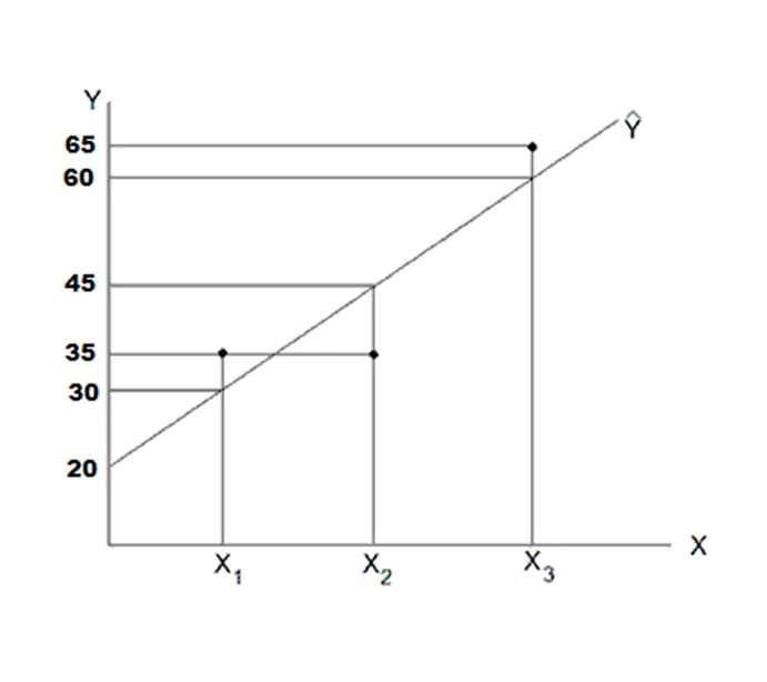
Diagram 1: An example of a filtered regression line
Question: Calculate the R^2 for the model associated with the above diagram.
Answer:
SSR=∑(Y-Y ̂ )^2
= (30-35)^2+(45-35)^2+(60-65)^2
=150
SST = ∑(Y-Y ̅ )^2 ,
Y ̅=(∑Y)/n=(30+45+60)/3=45
SST= (30-45)^2+(45-45)^2+(60-45)^2=450
R^2=1-SSR/SST
R^2=1-150/450=0.66667