Problem Description:
This R Programming assignment focuses on statistical distributions and confidence intervals, including concepts related to normal distributions, hypothesis testing, and various probability distributions. Additionally, it involves data manipulation and visualization in R.
Solution
Question 1: Statistical Distributions and Confidence Intervals
1.1 What is the 68-95-99.7 rule in a normal distribution? What determines the shape of a normal distribution?
Answer-The 68-95-99.7 rule in a normal distribution states that 68% of the data values falls within one standard deviation, 95% percent of data vales falls within two standard deviations, and 99.7% of data values falls within three standard deviations from the mean.The shape of a normal distribution is determined by standard deviation of normal distribution.
1.2 How does a type I error differ from a type II error? Which error is more concerning in your opinion? You may answer this question using some specific examples.
Answer- type I error is the probability of rejecting a null hypothesis even when it is correct and type II error is the probability of failing to reject a null hypothesis even when it is False. Type I error is more concerning because we may conclude that some effect or disease is there even though it is not there.
1.3 How do test statistics and p values help us make a decision when performing hypothesis testing?
Answer-By using test statistics we can check that weather a test statistics lies in critical region or not if it lies in critical region, we can reject the null hypothesis else not. Similarly by using p value we can check that weather p-value is less than significance level or not. If p-vale is less than significance level we can reject the null hypothesis else not.
1.4 Suppose you are interested in the average age of hundreds of millions of American voters who voted in the 2020 presidential election. You create a random sample and get a sample mean of 37 and a confidence interval of [33.7, 40.3] at the 95% confidence level. What does this confidence interval tell us about the average age of American voters?
Answer-We are 95% confident that average age of American voters lies in the interval [33.7, 40.3]
Question 2: Stats and Coding
This question will be based on the USAincome2021.csv data file. You will need to download this file from Blackboard and upload it to RStudio Cloud. Then you should use the read.csv() function to import the data file into RStudio workspace.
If you do not use RMarkdown to do your homework, make sure to copy and paste your results from RStudio into a Word document, or you will not receive due points.
3.1 Import the data file into RStudio and display the first 7 rows of the data frame.
>df<-read.csv("USAincome2021.csv")
> head(df,7)
| State | Income | |
| 1 | Alabama | 56929 |
| 2 | Alaska | 81133 |
| 3 | Arizona | 70821 |
| 4 | Arkansas | 50784 |
| 5 | California | 81575 |
| 6 | Colorado | 84954 |
| 7 | Connecticut | 80958 |
3.2 The values of the income variable are in USD. Creat a new variable by changing its unit of measurement into thousand dollars. You can name this new income variable as whatever you like. Display the first six values of this new income variable.
> df$income.in.thousand<-df$income/1000
> head(df$income.in.thousand,6)
[1] 56.929 81.133 70.821 50.784 81.575 84.954
3.3 Create a histogram to show the median household income measured in thousand dollars. Describe what the most common level of household income is in the United States.
> hist(df$income.in.thousand,breaks=10)
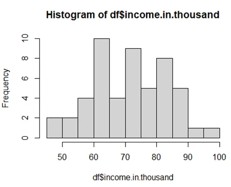
#the most common level of household income is in the United States lies in the interval 60-65k USD
3.4 Create a box plot to show the distribution of the median household income. Judging from the IQR (inter-quartile range), what is the median of the median household income in 2021? What is the size of IQR and what does it mean?
> boxplot(df$income.in.thousand,main="Boxplot of Household Income ($1000 USD)")
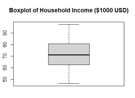
> #Median of household income
> median(df$income.in.thousand)
[1] 71.139
> #IQR of household income
> IQR(df$income.in.thousand)
[1] 17.9095
3.5 A pregnant woman is equally likely to give birth to a boy and a girl, which means that the probability of having a girl is 0.5 in the population. If you hear that someone has raised five kids, what is the probability that three of them are girls?
[You can earn 5 bonus points if you correctly answer the question by utilizing a formula and calculating the probability by hand]
> #By using Formula Manually
> p_girl<-0.5
> n_kids<-5
> n_girls<-3
> required_probability<-factorial(n_kids)/(factorial(n_girls)*factorial(n_kids-n_girls))*(p_girl)^n_girls*(1-p_girl)^(n_kids-n_girls)
> required_probability
[1] 0.3125
> #By using R function
> dbinom(x=3,size=5,prob=0.5)
[1] 0.3125
3.6 Suppose a newly developed missile could hit a target with a probability of 0.7. What is the probability that a target was hit after three missles were fired simultaneously?
[You can earn 5 bonus points if you correctly answer the question by utilizing a formula and calculating the probability by hand]
> #By using Formula Manually
> prob_success<-0.7
> n_trial<-3
> p_hit<-1-(1-prob_success)^n_trial
> p_hit
3.7 Suppose a random variable measuring the number of political parties in a country follows a Poisson distribuion, with a population mean (i.e., λ) of 5. If you randomly pick a country out of the 193 UN members, what is the probability that there are 7 political parties in this country?
[You can earn 5 bonus points if you correctly answer the question by utilizing a formula and calculating the probability by hand]
> #By using Formula Manually
> lambda<-5
> x<-7
> requiered_probability<-exp(-5)*lambda^(x)/factorial(x)
> print(requiered_probability)
[1] 0.1044449
> #By using R function
> dpois(x=7,lambda)
[1] 0.1044449
3.8 A random variable X follows a standard normal distribution. What is the probability that X takes a value of 1.23 at most? In other words, what is P(X≤1.23)?
> pnorm(1.23)
[1] 0.8906514
3.9 A random variable Z follows a Student’s t distribution with 38 degrees of freedom. What is the probability that Z takes a value not greater than -1.55? In other words, what is P(Z≤-1.55)?
> pt(-1.55, 38)[1] 0.06471544