Problem Description:
The Statistical Analysis assignment involves analyzing data from a wellness depression and anxiety program. The goal is to gain insights into the participants' age distribution, the effects of the program on depression and quality of life, as well as participants' qualitative responses to the program.
Solution
Univariate Analysis
For this analysis we chose the Age variable as a perfect ratio level data in the dataset. The mean value computed was (38.74, SD 5.89). This shows us that on average, the participants who participated in this survey were of 38 years of age. The median age value is 38 years and the modal age value is 40 years. The data was tested for outlier values and the results showed there were no outlier values. The range helped in determining the groupings of the data. The oldest participant in this survey was 52-year-old and the youngest was 27 years of age giving us a range of 25 years of age. The computed interval level for each frequency class was 4. The frequency distribution table is as shown below.
Table 1: Distribution table
| Grouped data | |
|---|---|
| Age | Frequency |
| 25-31 | 13 |
| 32-36 | 23 |
| 37-41 | 35 |
| 42-46 | 19 |
| 47-52 | 12 |
From this type of analysis of the data, I learnt that majority of the participants in this survey were aged between 37 years of age and 41 years of age. The study being a wellness depression and anxiety program, the data is relevant for these findings and can be used to draw insights. According to the WHO, the average age of onset for major depressive disorder is between 35 and 40 years of age which fits our data set. Having a wrong data set can lead to wrong conclusions and drawing misguided insights.
Bivariate analysis
Test 1
For test 1 we chose the Depression outcome test. The variables chosen were patient health questionnaire and the quality of life at different waves probably before and after depression to see the effect of depression on the quality of life. A paired t-Test for various sample means was used. The Student's t-Test is used to determine whether the null hypothesis (that the means of two populations are equal) can be accepted or rejected. The t-Test Paired Two Sample for Means tool conducts a paired two-sample analysis. The variances of both populations are not assumed to be equal in this test. Paired t-tests are commonly used to compare the means of a population before and after treatment.
The pre-test mean was 21.13 and the post-test mean was 11.51 for tests to assess the symptoms of depression (PHQ9). The percentage change is 45.53% from pre-test to post-test showing a reduction in the symptoms of depression for the PHQ9 wave 2. For this test we will use a two tailed t-Test. P (T <= t) two tail (1.77191E-53) gives the probability that the absolute value of the t-Statistic (31.055) would be observed that is larger in absolute value than the Critical t value (1.983731003). Since the p – value is less than our alpha, 0.05, we reject the null hypothesis that there is no significant difference in the means of each sample. And we conclude there is a significant difference in the sample mean of the pre-test and post-test. The findings suggest that the programs intervention helped in reduction of depression symptoms among these participants after the post-test wave 2.
For the quality of life, the pre-test mean was 27.31 and the post-test mean was 53.99. The percentage change is 97.69% from pre-test to post-test showing an increase in the Quality of life scale wave 2. For this test we will use a two tailed t-Test. P (T <= t) two tail (2.2075E-11) gives the probability that the absolute value of the t-Statistic (7.53) would be observed that is larger in absolute value than the Critical t value (1.983731003). Since the p – value is less than our alpha, 0.05, we reject the null hypothesis that there is no significant difference in the means of each sample. And we conclude there is a significant difference in the sample mean of the pre-test and post-test Quality of life scale. The findings suggest that the programs intervention helped in increasing the Quality of life among these participants after the post-test wave 2.
Test 2
For test 2, a two-sample t-test assuming unequal variances was used. It assumes that both groups of data are sampled from Gaussian populations, but does not assume those two populations have the same standard deviation. The variables used to see if there is a change in depression symptoms were No-work depression and Work depression. In this test, P (T <= t) two tail (0.861) gives us the probability that a value of the t-Statistic (0.1761) would be observed that is larger in absolute value than t Critical two-tail (1.991). Since the p-value is larger than our Alpha (0.05), we cannot reject the null hypothesis that there is no significant difference in the means of each sample. We conclude that there is no significant difference between participants who worked and experienced depression and those who did not work and experienced depression symptoms. This shows that work does not impact depression symptoms.
The variable used for quality of life was to see if there was a significant difference between quality of life in males and females. For this test, P (T <= t) two tail (0.84) gives us the probability that a value of the t-Statistic (0.210) would be observed that is larger in absolute value than t Critical two-tail (2.052). Since the p-value is larger than our Alpha (0.05), we cannot reject the null hypothesis that there is no significant difference in the means of each sample. Thus, we conclude that the there is no significant difference in the quality of life scale between males and females.
Qualitative analysis
For this analysis, we chose a code of scaling the responses into four main categories. 1= those who accept that they are getting better, 2= those who were hopeful that things would be okay, 3= those who are not sure if there was any change, and 4= those who say the study didn’t help at all. The frequency distribution of the responses is as shown below.
Table 2: Frequency distribution table
| Responses | Frequency |
|---|---|
| Getting better | 13 |
| I'm hopeful things will be okay | 18 |
| Not sure | 7 |
| It didn't help at all | 3 |
The data was visually analysed and the pie chart below shows the distribution of the responses.
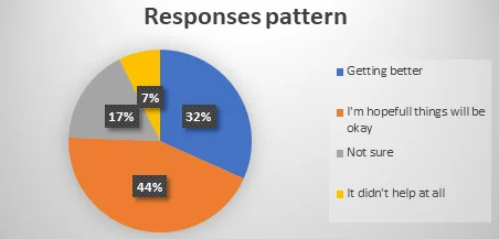
From the pie chart above, we can note that the study had an impact on both anxiety and depression symptoms since 76% of the participants agreed that things were either getting better or were hopeful things would get better for them whereas on 7% of the participants said the study didn’t help at all.